5 The main elements of an SDM
5.1 Objectives
This chapter will:
- Explore ideas of sampling effort under different data collection methodologies.
- Discuss minimal and more detailed ways of formatting data for modelling and prediction.
- Cast standard statistical modelling methods in the context of Species Distribution Modelling.
- Examine examples of specifying the likelihood of a model in frequentist and Bayesian platforms
- Examine examples of model structure (main effects, polynomials, interactions and their interpretation).
- Explore specialist elements of model selection and diagnostics pertaining to SDMs
- Interpret the coefficients of different types of SDMs
- Examine basic prediction techniques.
5.2 You are here
5.3 Representation of effort
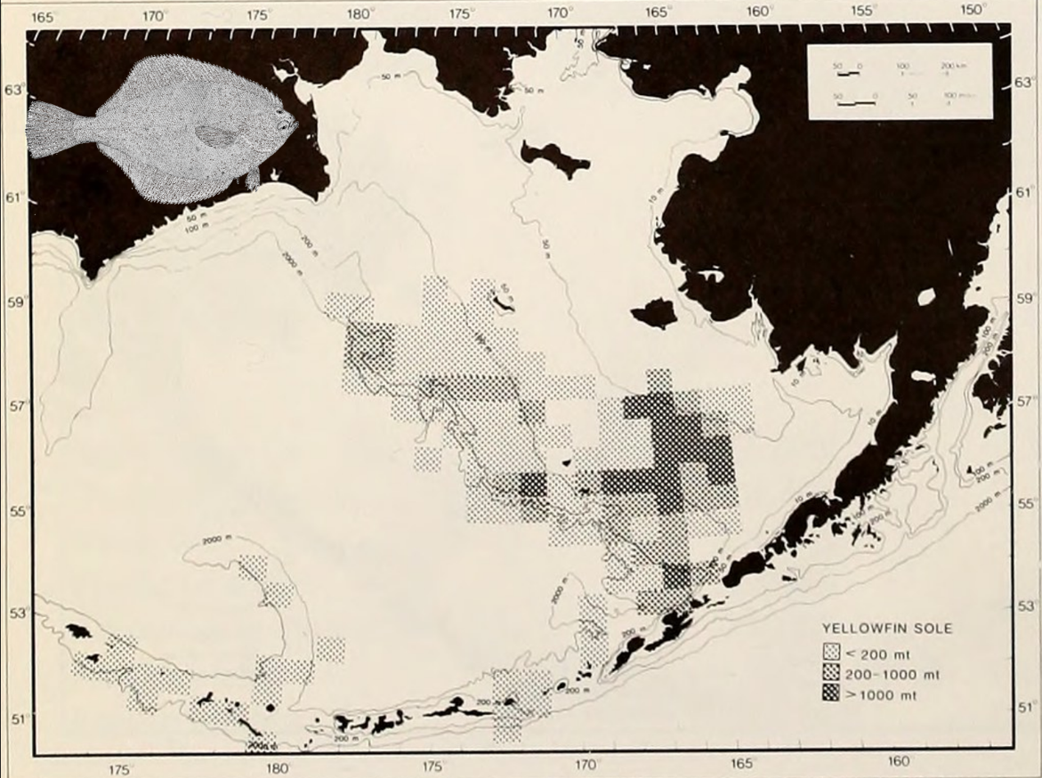
In fisheries science the most accessible form of spatial/temporal data on fish abundance are the reports by fishing vessels of catches in particular marine compartments (Figure 5.1)). Catch is usually reported as an estimate of the live weight of fish at capture, and it is tagged by vessel, trip and location. Using these data directly as a proxy of fish abundance is, of course, problematic for a number of reasons: Fish are often processed before they are weighted, the assignment of weights to species is not always perfect and many fish are often discarded back into the sea, to make room in the hold for more valued species, or to conform with fishing regulations. But most of all, catches are a biased proxy of abundance because fishing effort is almost never uniformly spread in space. Fishing vessels, particularly in small-scale fisheries, are essentially central-place harvesters whose effort is concentrated close to port, and in areas where skippers expect to have a good catch. The number and range of fishing vessels will fluctuate with fuel prices and salaries. Such biases, due to the economics of fishing or the behaviour of fishers can distort our view of the underlying abundance of fish.
The standard solution is to derive a measure of Catch Per Unit Effort, or CPUE, which is just the ratio of weight over fishing effort.
\[CPUE=\frac{Catch}{Effort}\]
If we are interested in modelling abundance, we can then go ahead and introduce some sort of regression model of CPUE as a function of covariates (e.g. bathymetry, or sediment). We are about to suggest that this approach is problematic, but let us momentarily follow this rabbit hole: We may use a linear model with a Gaussian likelihood, but this really does not deal well with CPUE values close to zero, and it can yield negative predictions which are patently not realistic. We could instead switch to a log linear model, but what likelihood should we use? CPUE is not going to take integer values (it will usually be mass rather than a fish count, and it is also a ratio), so a straightforward Poisson model may not be appropriate (and, it may also be underdispersed for real data). One solution is to round the CPUE data, but with small CPUE values, this might lose us a lot of information (turning them to zeros). Alternatively, we might use a log-linear model with a more exotic likelihood for non-negative and continuous values, such as the Gamma distribution. In R the model statement may look a bit like this:
model<-glm(CPUE~covariate1+covariate2, family=Gamma(link="log"))This approach is sensible, but we need to consider four challenges:
Definition of effort is hard: Fishing effort depends on time (how long did the vessel spend in an area?), fishing gear (how many hooks or how big a dredge?), and vessel speed (how much area did it cover?). Standardizing across different vessels is not straightforward. So, CPUE is a ratio with multiple denominators (e.g., catch per unit time, number of hooks and unit area)
Absolute abundance is elusive: Even if we could find some standardized unit of effort across the fishing fleet, we do not really have a parameterised functional response for fishing vessels - i.e. we generally lack a function that tells us how many fish will be caught per unit of effort as a function of the fish density at that location. Therefore, even if we can standardise the unit of effort, we cannot easily get to a measure of absolute abundance. This will be particularly problematic if the functional response is non-linear. E.g., the Holling type II functional response (Holling 1959) reaches an asymptote at high fish densities, meaning that the fishing gear becomes saturated with catch.
Zero effort cells give zero information: Although it is possible that the zero catch cells in (Figure 5.1)) are the result of no fish being there, they are just as likely a result of no fishing taking place. The ratio 0/0 is not defined numerically and this is why most modern plots would show these cells as NAs or missing values. In a process such as fishing, where the sampling effort is directed towards areas that are known or perceived to be high in abundance, the biology and its observation are deeply confounded.
Higher effort should represent higher precision: Even if the above three difficulties were countered somehow, representing abundance by CPUE hides a statistical weakness. Fundamentally, an area that has been fished a lot, is sampled a lot, and therefore, the estimated abundance is known with higher certainty than an area that a small vessel just happened to briefly cross into. A ratio of 1ton CPUE is the same whether one tonne was caught during a single unit of effort or 1000t were caught by 100 units of effort. Once we perform the division to arrive at the CPUE, we lose that information on precision.
The question of observation effort is perhaps the first an analyst must ask, once the response and explanatory data have been identified (see Chapter 4). It is handy to use the metaphor of trying to describe the distribution of the species across the landscape in the dark (lack of observations). It may be possible to flood the area with stadium lights (census) but in most cases our sources of light will be limited in some way. We may, for example, just have a torch. A survey can flash the torch at random places (grid sampling) or the surveyor can walk along straight lines, pointing the torch down in front of them (transects). Alternatively (stretching the metaphor to breaking point), we can try to flood the terrain with UV light, after having marked some of the individuals with fluorescent paint (telemetry). Finally, we might think of a generic point process as the random blinking of fireflies in the dark. Such a synoptic observation method is difficult to imagine at the moment, but it would correspond to very high resolution remote sensing images with advanced image recognition to identify the events of occurrence of the organisms of interest.
When you are preparing to analyse a spatial data set by a species distribution model, ask yourself: “Where is the effort processes in this study and what are its heterogeneities?”. If the answer is unclear, then red flags should go up. For example, in the case of CPUE, the effort is hiding in the denominator of the ratio. In general, for any analysis, it is much better practice to keep the data as close as possible to their raw form, even if this requires extending the features of the model a little to deal with multiple data types. For a fisheries model, it is better to ask for the raw catch and effort data separately, because we can exploit the offset facility of log-linear models. Mathematically, an offset can be thought of as covariate with a coefficient of 1. Here is why. Starting from the definition of CPUE, we can write the model as a loglinear function of the linear predictor:
\[\begin{eqnarray} \frac{\text{Catch}}{\text{Effort}} &=& exp(L(\textbf{x})) \\ \text{Catch} &=& \text{Effort}\exp(L(\textbf{x})) \\ &=& \exp(ln(\text{Effort})+L(\textbf{x})) \end{eqnarray}\]
Link to chapter 3 to discuss counts, surveys and use-availability.
5.4 Effort section
To investigate the effect of effort, let us create some toy data. Assuming that fish density is driven mainly by one covariate (cov) and that the effect of all other (unknown) covariates can be bundled into an error term (err), then we can write a habitat selection function for the true, underlying abundance in 100 grid cells on a hypothetical map. The relationship between the covariate and fish abundance is discernible by eye (Fig. 1a).
cells <-100
a0<--2
a1<-0.1
cov <- rnorm(cells,10,5) # A set of covariate values
err <- rnorm(cells,0,0.5) # Independent, random effects (e.g. by other covariates)
abn <- exp(a0+a1*cov+err) # True underlying abundance of fish
We simulate effort (eff- measured in some appropriate unit of hours/hooks etc.) via an exponential distribution and assume that it is unrelated to abundance (so, the skippers are really just hitting the shoals completely by chance). Then, we can model catches via some random process, such as the Poisson (but note that the overall outcome catch will be overdispersed by the effect of the err term, above).
eff <-rexp(cells,0.1) # Effort
catch <- rpois(cells,abn*eff)
These catches have a loosely linear association with the true underlying density of fish (Fig. 1c), which becomes better defined if they are plotted as CPUE against true density (Fig. 1d). However, the connection between CPUE and the covariate may be a little harder to see (compare Fig. 1d with Fig. 1b).
par(mfrow=c(2,2))
plot(cov, abn, main="a. True SHA", ylab="Fish density", xlab="Covariate")
plot(cov, catch/eff, main="b. Infered SHA", ylab="Catch/Effort", xlab="Covariate")
plot(abn, catch, main="c. Raw Catch v Truth", ylab="Catche", xlab="True density")
plot(abn, catch/eff, main="d. CPUE v Truth", ylab="Catch/Effort", xlab="True density")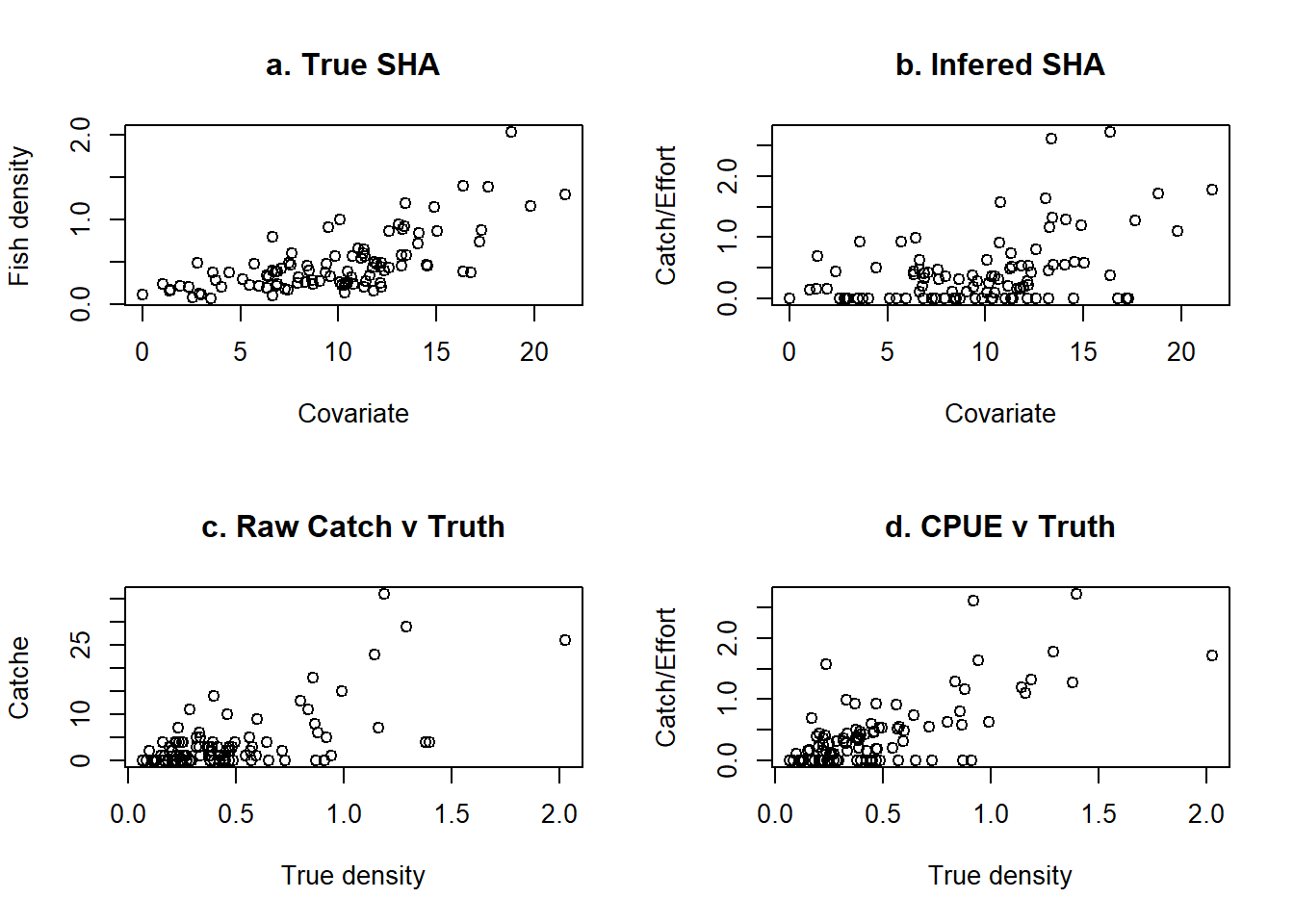
par(mfrow=c(1,1))- The true underlying density of fish, as a function of the single covariate, under the influence of stochasticity. b) The density that might be infered by looking at CPUE against the covariate. c) The raw catches of fish against the true fish density at each location and d) CPUE against the true fish density.
We will fit three models to tis data set. modelCPUE will use the ratio of catches over effort as the basis for the response variable. Because it is a linear model it will use the transformation log(CPUE+1) as the responce variable. The second model modelCatch uses the raw catch data as the response in a Poisson/log-linear model and offers the effort information as an offset. Finally, to investigate the overdispersion in the catch data, we use a negative binomial model modelCatchOD, a convenient alternative when the Poisson equidispersion assumption is suspect.
dat<-data.frame(catch,"cpue"=log(1+catch/eff), eff, cov)
modelCPUE<-lm(cpue~cov,data=dat)
modelCatch<-glm(catch~cov+offset(log(eff)), family=poisson, data=dat, maxit=50)
modelCatchOD<-glm.nb(catch~cov+offset(log(eff)), data=dat, maxit=50)
A summary of the parameter estimates from this model, compared to the true underlying parameters shows that the Poisson and NBinomial models approach both the true slope and the intercept and even thought their point estimates do not differ much, the NBinomial model’s confidennce intervals tend to bracket the true parameter values. The linear model in contrast is considerably worse. It might have been expected that the intercept a0 would be estimated with a bias, due to the addition of 1 in the transformed response variable (i.e. log(1+CPUE)). However, the slope estimate a1 is also biased.
| Parameter | CPUE | 95%CIs | Catch | 95%CIs | CatchOD | 95%CIs | True values |
| a0 | 0.01 | ( -0.13 , 0.15 ) | -2.25 | ( -2.55 , -1.97 ) | -2.13 | ( -2.57 , -1.7 ) | -2 |
| a1 | 0.03 | ( 0.02 , 0.04 ) | 0.13 | ( 0.11 , 0.16 ) | 0.12 | ( 0.09 , 0.16 ) | 0.1 |
Considerations of effort fall under the broader discussion of observation models, that were explored, for different data types, in Chapter 3. For instance, a general way of viewing the CPUE example is as a thinned Poisson process (see Section 3.8.2). This particular viewpoint allows us to think not just about the covariates driving the distribution, but also the covariates driving the effort of fishers. Two points on confounding that were made in that section bear some translation in the fisheries scenario. First, the non-identifiability of the intercepts of the biological process (representing the baseline density of fish) and the observation process (here, representing the catching efficiency of fishing effort). It is difficult to estimate how much of the resulting catch (per unit effort) is due to the average abundance of the fish and how much is down to the baseline catching efficiency of the fishing vessel. The second point was that when the biological and observation process depend on the same covariates, it may be difficult to separate them. In the fisheries example, as is the case with several citizen science, or safari/tourist-type observations, the “observers” try to go where the target species is. In a sense, the observation process is actively trying to read the same cues about the environment, making the confounding problems particularly acute.
5.5 The model-fitting data frame
A simple description of data structure, to make sure people are distinguishing this from the model prediction data frame.
5.6 The model likelihood
Close correspondence with families of distributions in GLM. Model fitting. Different frameworks, including likelihood, Bayesian, pieces of software available. Introductions to base-GLM, TMB, JAGS, INLA with example codes for a simple GLM. Note that we may choose to also discuss non-likelihood based approaches, such as MaxEnt or Machine learning (e.g. trees, forests). However, we could just refer readers to Guisan et al book for these.
5.7 Model structure
Main terms, polynomials, interactions, connections with Chapter 2.
5.8 Model diagnostics and model selection
General diagnostics and more specific diagnostics for SDMs Information criteria, shrinkage, spike-and-slab, model-averaging, cross-validation
5.9 Interpreting the coefficients
5.10 Prediction
Formulation of prediction data frame. Mean prediction. Uncertainty in predictions. Visualisation. Boostrapping methods.
5.11 Concluding remarks
5.12 References
Holling, Crawford S. 1959. “Some characteristics of simple types of predation and parasitism.” The Canadian Entomologist 91 (7): 385–98.